More than half of the Sun-like stars in the Milky Way belong to binary or multiple-star systems, and the catalogued variable stars now number over fifty-eight thousand (as of 2023). Binaries and variables transform stars from mere “points of light” into physical objects that can be studied quantitatively: the former provide almost the only means of directly measuring stellar mass, while among the latter the Cepheid variables and Type Ia supernovae form the key rungs of the cosmic distance ladder. This page distinguishes the criteria, physical mechanisms, and typical figures for the various classes of double and variable stars. Before reading, you may wish to review the fundamentals of stellar physics and the apparent magnitude system.
Two stars that appear very close together in the sky are called a double star. Their relationship has two possibilities:
Optical double / optical pair: the two stars merely happen to lie in nearly the same line of sight, while their actual distances differ enormously; they are not gravitationally associated and do not form a physical system.
Physical binary: the two stars are gravitationally bound and orbit their common center of mass (barycenter), forming a true binary system.
Telling the two apart requires proper motion, parallax, or long-term orbital motion: the two members of a physical binary share a common proper motion and trace an orbital arc over time, whereas the members of an optical double each go their own way.
Physical binaries are divided into four classes according to how they are discovered and observed. The same system may belong to several classes at once—for example, many spectroscopic binaries are also eclipsing binaries.
Type
English
Distinguishing criterion
Typical examples
Visual binary
visual binary
Resolvable by telescope into two separate stellar points
Sirius A/B, Mizar (Ursa Major)
Spectroscopic binary
spectroscopic binary
Spectral lines show periodic Doppler shifts due to orbital motion
Mizar A (Ursa Major)
Eclipsing binary
eclipsing binary
Orbit edge-on to Earth; members mutually eclipse, causing light variation
Algol (Perseus)
Astrometric binary
astrometric binary
Visible star wobbles about an empty point; companion invisible
Sirius B in the early days (before its discovery in 1862)
Visual binaries: the angular separation of the two members is large enough for a telescope to resolve them. The brighter is called the primary, the fainter the secondary. Orbital periods commonly range from decades to thousands of years, some exceeding ten thousand years.
Spectroscopic binaries: the two stars are too close to be resolved and can only be identified by the periodic redshift/blueshift of their spectral lines. There are two subtypes:
Single-lined spectroscopic binary (SB1): only the spectral lines of one member can be observed.
Double-lined spectroscopic binary (SB2): the spectral lines of both members are visible, alternating between single and double as the orbital phase changes.
Eclipsing binaries: the orbital plane is nearly coplanar with the line of sight, so the two stars mutually obscure one another, periodically reducing the total brightness; such a system is both a binary and a variable (see “Eclipsing variables” below).
Astrometric binaries: the companion is too faint to be seen directly, but its presence can be inferred from the periodic wobble of the primary relative to the background.
A gravitationally bound system with three or more members is called a multiple-star system. Stable multiple-star systems are usually hierarchical: members pair up into tight subsystems, and the subsystems in turn orbit one another in larger orbits, ensuring long-term dynamical stability.
Triple stars: θ¹ Orionis at the core of the Orion Nebula (commonly known as the Trapezium) is a famous multiple-star region.
Sextuple stars: Mizar and Alcor in Ursa Major together form a six-star system; Castor (Gemini) is likewise a sextuple star.
The central value of physical binaries is this: they provide almost the only means by which astronomers can directly weigh stellar masses. The two members orbit their common center of mass, and the distance from the barycenter to each star is inversely proportional to its mass:
r1 / r2 = m2 / m1
r1 = a · m2 / (m1 + m2)
Here a is the separation between the two stars, r1 and r2 are the distances of each star from the barycenter, and m1, m2 are the masses.
For a system with known orbital period P and semi-major axis a, Kepler’s third law gives the total mass of the system. In Solar System units, the formula takes its simplest form:
a^3 / P^2 = m1 + m2
where a is in astronomical units (AU), P in years (yr), and mass in solar masses (M☉). To further separate the individual masses of the two stars, one also needs: for visual binaries, the true scale from parallax together with the ratio of the two stars’ distances from the barycenter; for spectroscopic binaries, the radial-velocity curves; and for eclipsing binaries, the light curve, which additionally constrains the orbital inclination and the members’ radii.
Orbital periods span an enormous range: from less than an hour (e.g. AM CVn–type cataclysmic binaries), to a few days (e.g. β Lyrae), to several hundred thousand years (the orbit of Proxima Centauri about α Centauri AB). Statistically, binary periods approximately follow a log-normal distribution, with a median on the order of 100 years.
A variable star is one whose brightness changes with time. By the cause of variation they fall into two broad classes:
Extrinsic variables: the star’s own luminosity need not change; the brightness variation arises from geometric effects, such as members eclipsing one another (eclipsing variables) or rotation turning a non-spherical or spotted stellar surface alternately toward Earth (rotating variables).
Intrinsic variables: changes in the star’s own physical state cause the luminosity to change, including the three categories of pulsation, eruption, and cataclysm.
Among catalogued variables, pulsating types make up about two-thirds (nearly thirty thousand), and eclipsing variables number over ten thousand. The following sections proceed mechanism by mechanism.
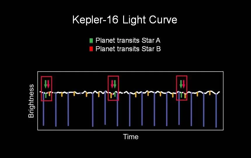
Eclipsing variables are the eclipsing binaries described above. The orbital planes of the two members lie close to the line of sight; when the fainter member obscures the brighter, the total brightness reaches a primary minimum, and conversely a shallower secondary minimum occurs. Algol (Perseus) is the prototype, with a light-variation period of about 2.87 days and a brightness varying between roughly magnitudes 2.1 and 3.4. The light variation of an eclipsing variable is entirely a geometric occultation effect, unrelated to the star’s internal physics, yet its light curve can be inverted to recover the members’ relative radii, brightness ratio, and orbital inclination.
Light curve of an eclipsing binary: a deeper primary minimum occurs when the fainter member eclipses the brighter, and a shallower secondary minimum when the brighter member eclipses the fainter, with brightness essentially constant between the two minima.
图源 NASA · Public domain
The historically famous “Algol paradox” refers to the fact that the less massive member of the system has in fact evolved faster (it has become a subgiant); the cause is that early mass transfer redistributed the masses of the two stars.
When a member is flattened into an ellipsoid by rapid rotation, or its surface bears large dark spots or bright patches, rotation periodically changes the effective emitting area or brightness facing Earth, producing a rotating variable. Among these, a star tidally distorted into an ellipsoid by binary interaction, whose projected area varies with orbital phase, is called an ellipsoidal variable, with a light-variation period equal to half the orbital period.
The outer layers of a pulsating variable expand and contract periodically under an imbalance between gravity and pressure, so that radius, temperature, and luminosity vary periodically as well. The energy source of pulsation is the kappa mechanism: a certain ionization layer inside the star (typically the second-ionization zone of helium) increases in opacity when compressed, trapping radiation and accumulating energy that drives the outer layers to expand; after expansion the temperature drops, the opacity falls back, radiation escapes, and the outer layers fall back, thus forming a heat-engine cycle. The temperature range that can sustain this mechanism forms a nearly vertical band on the Hertzsprung–Russell diagram, called the instability strip.
Type
English
Period range
Visual amplitude
Population / characteristics
Classical Cepheid
classical Cepheid
1–100+ days
about 0.1–2 mag
Population I, yellow supergiants, 4–20 M☉
W Virginis (Type II Cepheid)
Type II Cepheid
about 1–50 days
about 0.3–1.2 mag
Population II, old, about 0.5–0.6 M☉
RR Lyrae
RR Lyrae
about 0.2–1 day
about 0.2–2 mag
Population II, old horizontal-branch stars
Mira (long-period)
Mira / long-period
about 100–1000+ days
up to 8 mag or more
red giants / asymptotic giant branch
Semiregular
semiregular
tens to hundreds of days
usually < 2.5 mag
red giants / supergiants, period not strict
Cepheid Variables and the Period–Luminosity Relation
Classical Cepheids are high-luminosity yellow supergiants of 4–20 M☉, with luminosities up to one hundred thousand times that of the Sun. Their central rule is the period–luminosity relation (also known as Leavitt’s law): the longer the light-variation period, the higher the mean absolute luminosity, the two being approximately linear on a logarithmic scale. The relation was discovered by Henrietta Leavitt in 1908–1912 among the Cepheids of the Small Magellanic Cloud—because they belong to the same galaxy and lie at the same distance, the correspondence between period and apparent brightness directly reflects differences in true luminosity.
M = a · log10(P) + b
Here M is the absolute magnitude, P is the light-variation period (days), and a, b are empirical calibration constants (a is negative, so a longer period gives a smaller magnitude, i.e. brighter). Delta Cephei is the prototype of the classical Cepheids.
RR Lyrae: old, low-mass horizontal-branch stars with periods of about 0.2–1 day and a roughly fixed absolute magnitude (about +0.5 to +0.6 mag), serving as another class of standard candle for measuring distances to globular clusters and nearby galaxies.
Mira-type long-period variables (Mira): red giants taking Mira (Omicron Ceti) as their prototype, with periods of about 100 days to more than two thousand days and apparent-brightness changes of up to 8 magnitudes (a luminosity change of about a thousandfold).
Semiregular variables (semiregular): less regular than Mira types in both period and amplitude, with visual amplitudes usually below 2.5 mag, mostly red giants or red supergiants (Betelgeuse, for instance, exhibits closely related variable behavior).
A cataclysmic variable is a close binary containing a white dwarf: the white dwarf accretes material from a companion that fills its Roche lobe, and erupts under various conditions. Unlike supernovae, these eruptions do not destroy the progenitor star and can recur.
Type
English
Mechanism
Brightening / recurrence
Nova
nova
Thermonuclear flash once the hydrogen layer accreted on the white dwarf’s surface reaches a critical point
Brightens thousands to tens of thousands of times; long recurrence period
Recurrent nova
recurrent nova
Same as the nova mechanism; high accretion rate causes frequent eruptions
A supernova is the most violent of stellar-scale eruptions; its peak can brighten by more than 20 magnitudes within a few days, and for a short time its luminosity can rival that of an entire galaxy. They are classified by the presence or absence of hydrogen lines in the spectrum and further features, combined with the physical mechanism, as follows:
Type
Hydrogen lines
Key spectral features
Physical mechanism
Peak absolute magnitude (approx.)
Type Ia
absent
615 nm singly ionized silicon (Si II) line
Thermonuclear detonation of a white dwarf
−19
Type Ib
absent
No silicon; 587.6 nm neutral helium (He I) line present
Core collapse (hydrogen envelope already lost)
about −17
Type Ic
absent
No silicon; helium weak or absent
Core collapse (hydrogen and helium envelopes already lost)
A white dwarf in a close binary accretes material; as its mass approaches the Chandrasekhar limit (about 1.44 M☉), carbon burning ignites in a runaway, and the entire white dwarf undergoes thermonuclear detonation and is completely disrupted. The spectrum has no hydrogen but shows silicon lines. The energy released is about 1–2×10⁴⁴ joules, and the ejecta travel at about 5000–20000 km/s.
Core-collapse supernovae (II / Ib / Ic)
A massive star of about 8 M☉ or more evolves to an iron core; nuclear fusion can no longer resist its own gravity, the iron core collapses and violently rebounds in an explosion. Depending on whether the hydrogen and helium outer layers are retained before the eruption, it appears as Type II, Ib, or Ic. After the explosion a neutron star or black hole usually remains at the core.
Because their detonation conditions (near the Chandrasekhar limit) are highly uniform, Type Ia supernovae have a nearly standardized peak luminosity (about −19 mag), and after correction for light-curve shape they can serve as standard candles at extreme distances. In 1998, it was precisely by using high-redshift Type Ia supernovae that two independent teams discovered the universe to be in a state of accelerating expansion, on the basis of which dark energy was proposed.
The material ejected by the explosion expands at thousands to tens of thousands of kilometers per second, colliding with the interstellar medium, being heated by the shock wave, and emitting light to form a supernova remnant. The Crab Nebula (M1) in Taurus is the remnant of the supernova of AD 1054 (SN 1054), and at its center remains a rapidly rotating neutron star (a pulsar).
Within a single constellation, variable stars are labeled in order of discovery using the Bayer-style variable-star nomenclature (stars that already have a Bayer Greek-letter name keep their original name):
First batch: capital letters R through Z (9 per constellation).
Then: RR–RZ, SS–SZ … up to ZZ, and on to AA–AZ … QQ–QZ (omitting the letter J).
Once these 334 combinations are exhausted, numbering switches to V335, V336 … in order of discovery.
For example, Algol’s variable-star name is “β Persei” (keeping its Bayer name), while RR Lyrae, ο Ceti (Mira), and others are each named according to the rules.
A curve recording the change in brightness over time is called a light curve, with magnitude on the vertical axis (brighter upward) and time on the horizontal axis. For a variable of known period, the time can be folded by the period and a magnitude–phase diagram plotted with phase (0–1) on the horizontal axis, superposing data from many periods onto a single curve, which makes it easier to precisely measure the period, amplitude, and times of minimum.
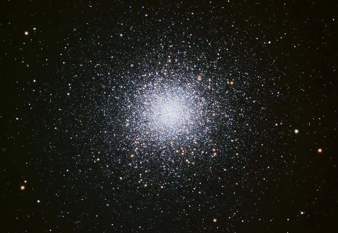
Globular clusters are ideal places for practicing variable-star observation (especially RR Lyrae): the members within a cluster lie at essentially the same distance, making it easy to compare brightness side by side. Observing methods can be combined with this site’s hemisphere visibility and observing conditions to plan targets.
The globular cluster M13 in Hercules: gathering hundreds of thousands of stars and containing several classes of variables, it is a classic target for variable-star surveys and brightness comparison.
图源 Sid Leach/Adam Block/Mount Lemmon SkyCenter · CC BY-SA 4.0
Use the apparent magnitude system and comparison stars of known brightness within the field to estimate brightness visually.
Record the brightness of Algol, Mira, and others over the long term, plot the light curves, and superpose them into a phase diagram to determine the period.
Binary star — Wikipedia: observational classification of binaries (visual / spectroscopic / eclipsing / astrometric), Roche-lobe classification, and the mass-determination formula.
Variable star — Wikipedia: the intrinsic/extrinsic classification scheme for variables, naming rules, and catalogue statistics.
Cepheid variable — Wikipedia: the Cepheid period–luminosity relation (Leavitt’s law), the kappa mechanism, and the application as standard candles.
Supernova — Wikipedia: supernova classification by spectrum and mechanism into Ia / Ib / Ic / II, peak luminosity, and energy data.
Types of Variable Stars — AAVSO: the American Association of Variable Star Observers’ beginner-level summary of periods and amplitudes for the various classes of variables.