Sensors: CMOS / CCD / Mono / OSC
The image sensor is the device that converts incident photons into a quantifiable electrical signal, and it is the heart of an astronomy camera. Several of its physical metrics—quantum efficiency, read noise, dark current, full well capacity, and pixel size—together determine what signal and noise a camera can record under long exposures. This page first introduces the two sensor architectures (CMOS and CCD) and the two color-capture methods (monochrome and color), then explains the key performance parameters one by one, and finally distinguishes the roles of three classes of equipment: dedicated astronomy cameras, modified DSLRs/mirrorless cameras, and planetary cameras. Understanding these parameters helps you make quantitative judgments when purchasing, planning a shoot, and processing, and the related concepts can be cross-referenced with signal-to-noise ratio and optics fundamentals.
The basic working process of a sensor
Section titled “The basic working process of a sensor”Whether CMOS or CCD, the basic physical process is the same:
- Photoelectric conversion: incident photons excite photoelectrons in a silicon photodiode via the photoelectric effect, and the electrons are collected and stored in the potential well of a pixel. Whether an electron is produced is determined by the quantum efficiency (QE).
- Charge accumulation: during the exposure the pixel continuously accumulates electrons until the number of accumulated electrons reaches its ceiling, the full well capacity.
- Readout: after the exposure ends, the charge is converted to a voltage, then quantized into a digital reading by an amplifier and an analog-to-digital converter (ADC), in units of ADU (analog-to-digital unit).
- Noise addition: the readout process introduces read noise; thermal motion during the exposure produces dark current.
The fundamental difference between the two types of sensors lies in step 3—how the charge is read out.
CMOS versus CCD
Section titled “CMOS versus CCD”A CCD (charge-coupled device) uses an analog shift-register structure: after the exposure, the charge of each row is “transferred” row by row to the few amplifiers at the edge of the chip, where it is uniformly converted to a voltage. The entire chip shares the same readout chain, which gives extremely high uniformity but slow readout.
A CMOS (complementary metal-oxide-semiconductor) sensor is an active-pixel sensor (APS): each pixel has its own amplifier circuit, the charge is converted to a voltage locally at the pixel, and rows can be read out in parallel. This greatly increases readout speed and lowers power consumption and heat generation.
Early CMOS sensors had a low fill factor and low QE because each pixel’s amplifier circuit occupied light-sensitive area, and inconsistency among the per-pixel amplifiers introduced fixed pattern noise (FPN). Over the past decade or so, the back-side illumination (BSI) process has moved the wiring layer to the back of the photodiode and, combined with microlenses for light concentration, has brought QE level with or even above that of CCDs; mature manufacturing has also reduced read noise to the 1–3 e⁻ range. Today CMOS has become the absolute mainstream in astronomy, and CCD has essentially exited the new-product market.
| Comparison item | CMOS | CCD |
|---|---|---|
| Readout structure | Each pixel has its own amplifier, parallel readout | Charge shifted row by row to edge amplifiers |
| Read noise | Low, can be as low as about 1 e⁻ | Relatively low and uniform, usually about 5–15 e⁻ |
| Readout speed | Fast, suited to planetary work and short-exposure stacking | Slow |
| Power consumption and heat | Low | High |
| Full well capacity | Smaller (with small pixels) | Usually larger |
| Amp glow | Present in older models, mostly eliminated in new ones | Almost none |
| Status and price | Mainstream, good value | Relegated to niche/used market, gradually discontinued |
Monochrome versus color (OSC)
Section titled “Monochrome versus color (OSC)”Astronomy cameras are divided into two types by color-capture method: monochrome (mono) and color (one-shot color, OSC).
The Bayer array and demosaicing
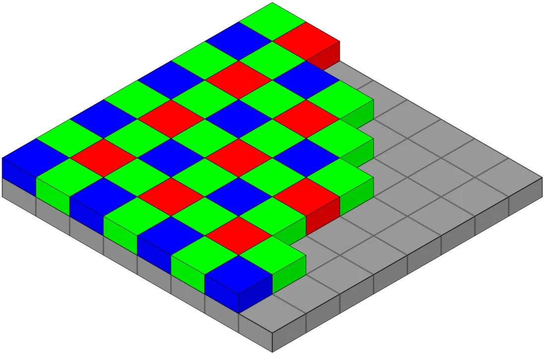
Section titled “The Bayer array and demosaicing”A color camera covers the sensor surface with a Bayer filter array: a red, green, or blue micro-filter is placed over each pixel, arranged in an RGGB pattern with a 2×2 repeating unit, in which green makes up 50% and red and blue 25% each. The higher proportion of green is meant to match the human eye’s greater sensitivity to brightness (which is determined mainly by green light).
Because each pixel records only one color, a demosaicing (also called debayer) algorithm is needed to interpolate the other two color channels missing from each pixel from neighboring pixels, in order to reconstruct a full RGB image. In high-contrast regions such as edges, demosaicing can produce artifacts such as false color, zippering, and moiré.
The trade-offs between mono and OSC
Section titled “The trade-offs between mono and OSC”A monochrome camera has no Bayer array, and all pixels receive the full spectrum, so the signal captured per unit area is higher than that of a color camera (in a color camera, about 2/3 of the spectrum is blocked at each pixel by the micro-filter). To produce a color image, a monochrome camera needs a filter wheel to shoot the L (luminance), R, G, B channels or narrowband channels (such as Hα/OIII/SII) one by one and then combine them. This delivers higher sensitivity, resolution, and narrowband capability, at the cost of greater equipment cost (camera + filter wheel + multiple filters) and more shooting and processing effort.
In practice, a good OSC camera used to its full potential can reach about 80% of the imaging quality of a monochrome setup; closing the remaining gap requires extra investment in time and budget. OSC produces a color image in a single exposure and needs fewer total frames, which is more advantageous when usable clear nights are short or the site is constrained.
| Comparison item | Mono + filter wheel | Color OSC |
|---|---|---|
| Color-capture method | All pixels receive light, shot channel by channel then combined | Single exposure with Bayer array then demosaiced |
| Signal utilization | High (no micro-filter blocking) | Lower (only one color per pixel) |
| Effective resolution | High (no color interpolation) | Slightly lower (reconstructed by interpolation) |
| Narrowband imaging | A strong point (can shoot SHO/HOO per channel) | Limited (requires dual-narrowband filters) |
| Ease of producing an image | Low (multiple channels + combining) | High (single exposure) |
| Equipment cost and workflow | High, complex workflow | Low, simple workflow |
| Suited to | Advanced users seeking image quality, narrowband | Beginners, portability, under urban light pollution |
If you plan to delve into narrowband imaging (Hα/OIII/SII), monochrome with narrowband filters is usually the necessary path; see narrowband imaging for details.
Key performance parameters
Section titled “Key performance parameters”Quantum efficiency
Section titled “Quantum efficiency”Quantum efficiency (QE) is the proportion of incident photons the sensor converts into usable photoelectrons, expressed as a percentage, and it varies with wavelength (the peak QE is usually quoted). The higher the QE, the more sensitive the sensor. Modern back-side-illuminated CMOS can reach a peak QE of 80%–91%, while front-side-illuminated sensors are around 50%–70%.
Read noise
Section titled “Read noise”Read noise is the random noise introduced each time a pixel is read out, in units of electrons (e⁻). It is independent of exposure length and is added to every frame. The lower the read noise, the better one can approximate the result of a single long exposure with “stacking many short exposures,” and the more one can reduce the per-frame exposure time to cope with tracking errors or light pollution. Modern CMOS read noise is often in the 1–3 e⁻ range.
Dark current and cooling
Section titled “Dark current and cooling”Even in the absence of light, thermal motion in the silicon material continuously generates electrons, namely dark current, often in units of e⁻/pixel/second. Dark current grows roughly exponentially with rising temperature (roughly doubling for every 6–7°C increase), becoming worse with longer exposures and higher temperatures, and it is accompanied by random thermal noise.
A cooled camera uses a thermoelectric cooler (TEC, i.e., a Peltier element) to bring the sensor temperature below ambient, typically by a margin (ΔT) of 30–40°C, and a PID algorithm stabilizes the temperature at the set value (to an accuracy of 0.1°C). Cooling serves two purposes:
- Suppressing dark current and thermal noise, markedly improving the long-exposure signal-to-noise ratio;
- Locking to a fixed temperature, allowing a library of dark frames to be built and reused long-term—dark-frame subtraction depends on temperature consistency, and this is precisely the key advantage of a cooled camera over an uncooled one.
Full well capacity and dynamic range
Section titled “Full well capacity and dynamic range”Full well capacity is the maximum number of electrons a single pixel can hold before saturating, in units of e⁻, and it determines how much light a pixel can record without overexposing. The larger the pixel, the larger the full well usually is.
Dynamic range is the ratio of the faintest to the brightest signal that can be recorded simultaneously, reflecting a frame’s ability to keep both shadow detail and highlights from clipping. Its approximate formula is:
dynamic range (dB) ≈ 20 × log10(full well capacity ÷ read noise)
It can also be expressed in stops: dynamic range (stop) ≈ log2(full well capacity ÷ read noise). Increasing the full well or lowering the read noise both widen the dynamic range.
ADC bit depth and gain modes
Section titled “ADC bit depth and gain modes”The ADC bit depth determines how many gray levels each pixel’s voltage is quantized into. Common values are 12-bit (4096 levels), 14-bit, and 16-bit (65536 levels). Insufficient bit depth produces posterization in smooth gradients.
Gain controls how many ADU correspond to a unit of electrons (i.e., the electron-to-ADU conversion ratio, e⁻/ADU). Raising the gain can lower the effective read noise, but it shrinks the usable full well and compresses the dynamic range. Many modern CMOS sensors offer dual conversion gain:
| Mode | Meaning | Characteristics and uses |
|---|---|---|
| HCG | High conversion gain | Lower read noise and better dynamic range, suited to faint targets and narrowband |
| LCG | Low conversion gain | Larger full well, suited to bright targets and preventing highlight saturation |
Cameras often switch automatically from LCG to HCG at a certain gain threshold, balancing low read noise and a large full well around that point.
Pixel defects and fixed pattern noise
Section titled “Pixel defects and fixed pattern noise”- Hot pixel / dead pixel: individual pixels that, due to manufacturing defects or unusually high dark current, read out abnormally high (hot pixel) or constantly low (dead pixel) even in the absence of light. Hot pixels increase with temperature and exposure length and are a repeatable signal that can be calibrated with a dark frame or a bad pixel map.
- Fixed pattern noise (FPN): a spatially fixed pattern caused by inconsistencies among per-pixel amplifiers and gains, which can be reduced through flat-frame and dark-frame calibration.
Pixel size, sampling rate, and binning
Section titled “Pixel size, sampling rate, and binning”Pixel size (in μm) and the telescope’s focal length (in mm) together determine the sampling rate (also called image scale)—the angle of sky each pixel corresponds to, in arcseconds per pixel (″/px):
sampling rate (″/px) ≈ 206.265 × pixel size (μm) ÷ focal length (mm)
Pixels that are too small relative to the optical resolution and seeing lead to “oversampling,” where each pixel collects little light and the per-frame signal-to-noise ratio drops; pixels that are too large lead to “undersampling,” which loses resolution detail. Deep-sky imaging often takes 1″–2″/px as a reasonable range (depending on seeing and guiding accuracy). For the relationship between pixels, focal length, and field of view, see optics fundamentals.
Binning combines adjacent N×N pixels into a single larger “super pixel,” trading resolution for signal-to-noise ratio:
| Type | Implementation | Characteristics |
|---|---|---|
| Hardware binning | Charge combined on-chip before readout (typical of CCD) | Read noise is counted only once, the largest SNR gain, faster |
| Software binning | Pixels summed/averaged in the data after readout (common with CMOS) | Flexible, can be done in post, but read noise is counted per pixel individually |
CMOS usually uses software binning, whose SNR improvement is not as significant as CCD hardware binning, but it can still raise the per-frame signal-to-noise ratio and frame rate when undersampling is acceptable, which helps on narrowband or poor-seeing nights.
The roles of three classes of cameras
Section titled “The roles of three classes of cameras”| Type | Main characteristics | Suited uses |
|---|---|---|
| Dedicated astronomy camera | With TEC cooling, high QE, mono/OSC variants, can take a filter wheel | The mainstay for deep-sky long exposures |
| DSLR/mirrorless | General-purpose and portable, no cooling, built-in Bayer color | Beginners, wide-field starscapes, the Milky Way, constellations |
| Planetary camera | High frame rate, small pixels, usually no cooling, can crop a region of interest (ROI) | Planets, lunar “lucky imaging” |
Dedicated astronomy cameras are optimized for long exposures: cooling suppresses dark current and allows a dark-frame library to be built, and monochrome models with a filter wheel can do narrowband, making them the mainstay tool for deep-sky work.
DSLRs/mirrorless cameras are general-purpose and portable, but the factory IR-cut filter (also called a hot mirror) greatly attenuates the 656 nm Hα red light, making emission nebulae appear weak; they also have no cooling, so thermal noise is noticeable in long exposures. Astro-modification refers to replacing or removing this filter: a typical modification raises the Hα transmission from about 22% to about 90% (about 4×), markedly enhancing the rendering of emission nebulae; but after modification, daytime shooting requires adding a color-correction filter, and the manufacturer’s warranty is voided.
Planetary cameras are optimized for short exposures and high frame rates: small pixels and fast readout, and a small region of interest (ROI) can be cropped to speed up further, usually with no cooling (dark current has little effect under short exposures). They work by “lucky imaging”—recording video at tens to over a hundred frames per second, then afterward selecting and stacking the few sharp frames in which atmospheric turbulence was momentarily steady, to counter seeing jitter.
Once you have a clear grasp of the sensor’s architecture and parameters, you can string optics (focal length, aperture), exposure (gain, per-frame duration), and post-processing (dark- and flat-frame calibration, stacking) into a complete chain. You can return to photography fundamentals, or proceed to getting started with capture.
References
Section titled “References”- Image sensor — Wikipedia: basic concepts such as the CMOS active-pixel sensor and CCD shift-readout principles, the back-side-illumination process, dynamic range, and noise.
- Bayer filter — Wikipedia: the Bayer array RGGB arrangement, the rationale for green at 50%, demosaicing, and common artifacts.
- CCD vs. CMOS Detectors in Astronomical Photometry — ICO Optics: a comparison of CMOS and CCD in astronomical applications across QE, read noise, amp glow, and pixel size.
- Quantum Efficiency, Read Noise, and why they are important — Altair Astro: definitions and typical values of QE, read noise, gain, and bit depth.
- Astro Cameras: OSC vs. Mono — Cosgrove’s Cosmos: real-world trade-offs between monochrome and OSC in signal utilization, narrowband capability, and workflow.
- What Is An Astro Modified DSLR Camera? — Skies & Scopes: the principle of DSLR astro-modification and quantitative data on the Hα transmission improvement.